Solving the Joint Order Batching and Picker Routing Problem for Large Instances

A summary of the methods employed and results obtained for the project undertaken in partial fulfillment for the degree of Bachelor of Science with Honours in Applied Mathematics at the National University of Singapore.

Acknowledgements

I would like to thank my industrial supervisor, Dr Melvin Zhang from The Intelligent Warehouse for his patience, guidance and knowledge. His insights have greatly strengthened the findings of this project.

Abstract

In this work, we investigate the problem of order batching and picker routing in warehouse storage areas. These problems are known to be capital and labour intensive, and often contribute to a sizable fraction of warehouse operating costs. Here, we consider the case of online grocery shopping where orders may consist of dozens of items.

We present the problem introduced in [1] and tackle the issue of solving the problem heuristically with proposed methods of solving that utilize batching and routing heuristics. Instances with up to 50 orders were solved heuristically in large simulated warehouse instances consisting of 8 to 30 aisles, with 1 to 4 blocks. The proposed methods were shown to have relatively short computation times as compared to optimally solving the problem in [1]. In particular, we showed that a proposed method which utilizes an optimal solver for routing yielded poorer results than methods that utilize routing heuristics.

Keywords: integer programming, inventory management, order batching, order picking, picker routing

Methods Employed in Solving

ILP Solver

To obtain optimal solutions to the ILP formulation, we employed a branch-and-cut solver to solve the formulation written in MiniZinc, an open-source constraint modeling language.

Method 1

In this method, we first compute the order batching via the time savings heuristic (TSH) [2]. Picker routing heuristics were used to obtain estimates of the partial route distances, for use in the TSH. Partial routes were computed by running each of the following heuristics: Nearest Neighbor, S-shape and Largest gap.

Method 2

This method involves the use of a heuristic with optimal routing for the final assignment of orders. In other words, we use the routing estimates obtained during the routing algorithms in the TSH (to batch orders), but once all orders have been assigned (batched), we solve for each picker optimally to find its optimal route.

For our experiments, in the order batching stage of Method 2, we employ the TSH which uses the routing heuristics introduced in Method 1. Then once order batches are computed in Python 3, to solve for each picker’s route optimally (with their batched order), we employ the Concorde TSP Solver. In particular, once orders have been batched to each picker, the JOBPRP is equivalent to the general TSP problem [7] as picker capacities have already been handled in the routing heuristics in the TSH.

Method 3

Here, instead of using routing heuristics to compute the routing estimates in order batching and routing of pickers after final assignment of batched orders, we employ the Concorde TSP solver [9] to compute optimal routes.

Data Files

The results obtained from experimenting with the above methods are found in the results folder, where results for the ILP solver (exact solving) are found in .exact files, and results for Methods 1 to 3 are found in .csv files.

Types of Data Files

.exact: Output from exact solving with CBC solver with the MiniZinc constraint model.

trivialbatching_<...>.csv: Results from solving without batching involved (i.e. 1 order to 1 picker), and using the PyConcorde TSP solver for picker routing. The results from this is used in the computation of the quality of solution.

320_picker_capacity_<...>_test-results.csv: Results from solving with Methods 1 to 3. The results from this is used in the computation of the quality of solution.

Interpreting the Variables in the Datasets

Method Used: Labelled as Methods 1 to 3.

Number of Orders: Number of orders for that test instance, where items in orders need not be distinct.

Objective Value: The total distance traversed by all the pickers combined from routing them with their batched order.

Time Elapsed (s): The time taken to compute batching of orders and routing of pickers.

Time Savings Router: The heuristic used in computing savings. Here, we have nn - Nearest Neighbor, sshape - S-shape, lgap - Largest Gap, concorde - PyConcorde.

Order Batch Router: The heuristic used in routing pickers once orders have been batched. Similarly, we have nn - Nearest Neighbor, sshape - S-shape, lgap - Largest Gap, concorde - PyConcorde.

Order File: The order file generated from Foodmart Database.

Order Size: Number of days worth of orders from a unique customer combined together. The days are 5, 10, 20.

Number of Aisles: The number of Aisles in the warehouse instance.

Number of Extra Cross Aisles: The number of cross-aisles partitioning the warehouse into blocks. For e.g., a warehouse with 1 block has 0 extra cross aisles, and a warehouse with 2 blocks has 1 extra cross aisle. Note that the number of extra cross aisles is equal to the number of blocks - 1.

Number of Shelves: Number of shelves stacked vertically per pallet.

Number of Products: Number of distinct products in the warehouse.

Picker Capacity: Picker capacity for the test instance.

Number of Pickers: Number of pickers required to pick all items from the batched orders. Note that each picker is assigned only to 1 batched order.

Results

Exact Solving

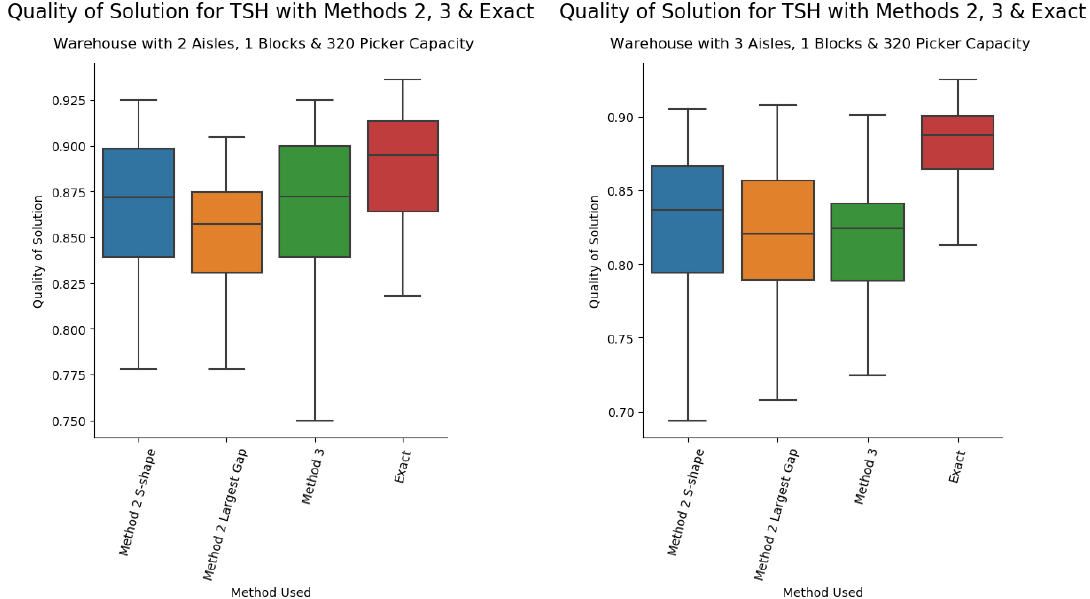
For exact solving, with a solver time limit of 1 hour, we were only able to obtain results with sufficient data points for small warehouse instances with 2 and 3 aisles. From the plots of their quality of solution, we observed that as the number of aisles increases, the gap between the median quality of solution for exact solving and heuristic solving with Methods 2 and 3 increases. No other generalizations can be made from the results obtained at the moment.

Heuristic Solving for Large Instances

From the results obtained from heuristic solving with Methods 1 to 3, we made some general observations across all large warehouse instances, the first being that Method 1 Nearest Neighbor is the fastest (with lowest median time) across all blocks. This is not highly unusual, as in our implementation of the Nearest Neighbor router, there was no sequence of nodes (node_sequence) to visit which contained several other nodes that are not pick nodes (like in S-shape and Largest Gap routers). This reduced the need for extensive computation of shortest paths, hence resulting in a significantly lower time to compute routes. The Nearest Neighbor router in Method 1 also resulted in the best (lowest) median objective value across all the other routers used in Method 1, except for 3 out of 16 results for Method 1. Note that the Nearest Neighbor heuristic is not used in practice in general, as actual aisles can be very narrow and it does not make sense for the picker to perform a u-turn in that narrow aisle, especially when the picker has a cart with them to store picks.

Another important observation is that across all large warehouse instances and across all blocks, Method 2 (with its resp. routers) has a lower median objective value than Method 1 (with its resp. routers). This result is in line with the fact that using an optimal router instead of a routing heuristic for routing of pickers should give a objective value less than or equal to that of the routing heuristic. Thus, we decided to analyze only results from Methods without the Nearest Neighbor heuristic as a router, and excluded Method 1 from our analysis as its results were poorer than Methods 2 and 3.

To gain deeper insights on the results obtained for the total distance traveled by the pickers, we plotted the box plots of quality of solution against the method of solving used for each large warehouse instance and for 320 picker capacity. The box plots are of the form:

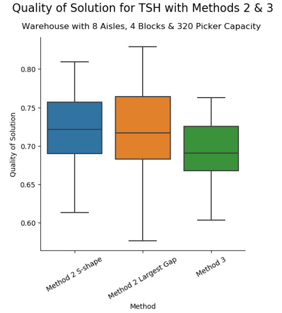
One interesting yet perplexing observation we made was that there are methods with a higher median quality of solution and lower spread than Method 3. An example can be found in the figure above, where Method 3 has a lower median quality of solution than Method 2 with S-shape and Largest Gap router. This result is counter-intuitive as a natural thought will be that Method 3, having both savings and batch router to be optimal routers, should yield a higher quality of solution than all methods that employ routing heuristics in solving. Our interpretation of this result is that using a routing heuristic instead of an optimal router as savings router can result in batching being performed in such a way that the overall objective value will be lower than in the case where an optimal router is used as savings router.

To gain a deeper insight as to what happened during the batching for Methods 2 and 3, we plotted the batches and routes for the test instance which had Method 2 with a higher quality of solution than Method 3. The following is an example of one such test instance with 10 orders where Method 2 with S-shape has a higher quality of solution than Method 3:

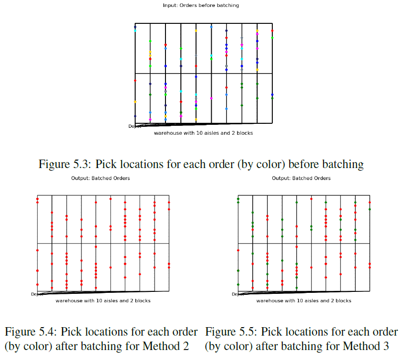
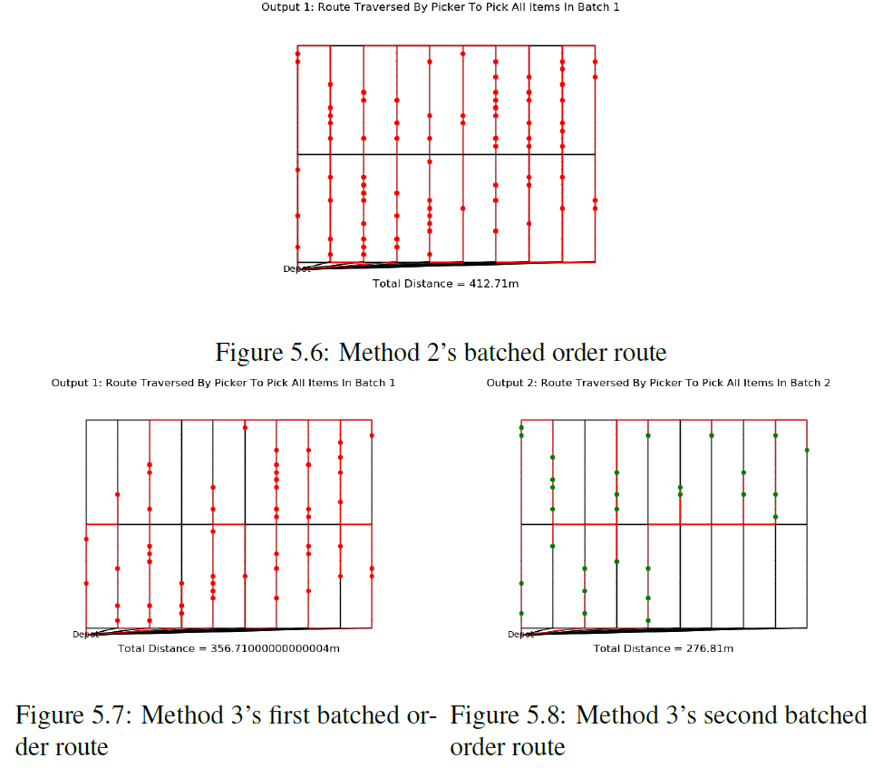
In this test instance, we observed that for an input with 10 orders, Method 2 S-shape produced 1 batched order as output whereas Method 3 produced 2 batched orders as output. Furthermore, when these batched orders have been routed with the respective batch routers, the total distance traveled by the pickers across all the routed batched orders in Method 3 is more than that of Method 2 S-shape. The following plots in Figures 5.6, 5.7 and 5.8 illustrates this.

At this stage, we are not able to draw anything conclusive, so we decided to look into the critical point in the batching process where a new batch was formed for Method 3. Denote the orders by their indices from 1 to 10. Then we obtained the batched orders - for Method 2 S-shape: Batches = [[3,4,1,5,9,10,2,6,8,7]] and Method 3: Batches = [[3,4,1,2,8,7], [5,10,6,9]]. Next, we computed the savings matrix for Method 2 S-shape and Method 3:

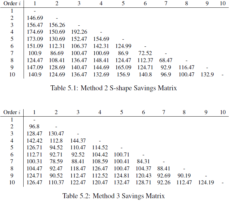
So what happened during the batching? To find out more, we computed the steps of the batching, where we found that order 5 does not get added to the first batch of orders at the third step:

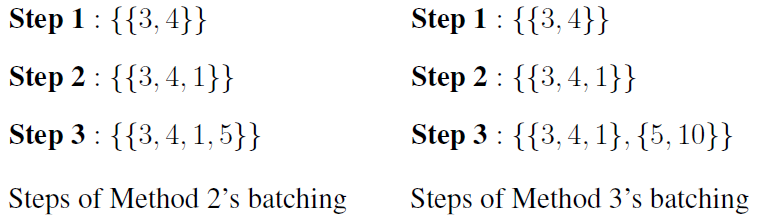
To analyze this critical step deeper, we refer to the savings matrix for Method 3:

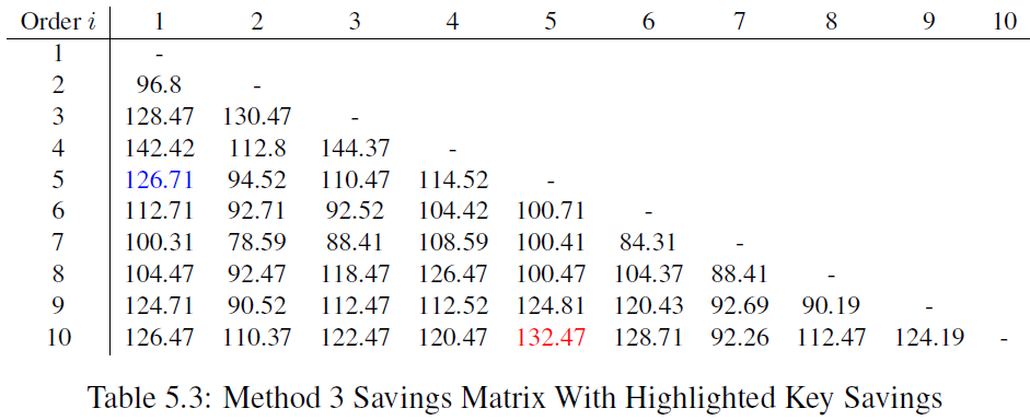
In the third step for Method 3, we observed that order pair (5, 10) had a higher savings than (1, 5) in the third step. On the contrary for Method 2 S-shape, it can be seen from Table 5.1 that order pair (5, 10) had a lower savings than (1, 5). As a result, a new batch is formed for order pair (5, 10) in step 3 for Method 3, which ultimately lead to a higher total distance traveled for Method 3.

We also computed the median time elapsed for each method of solving, by combining all same methods of solving with the S-shape and Largest Gap routers together. For e.g., we analyzed the results of Method 1 with S-shape, Largest Gap for the savings router together. We obtained the following plot as a result:

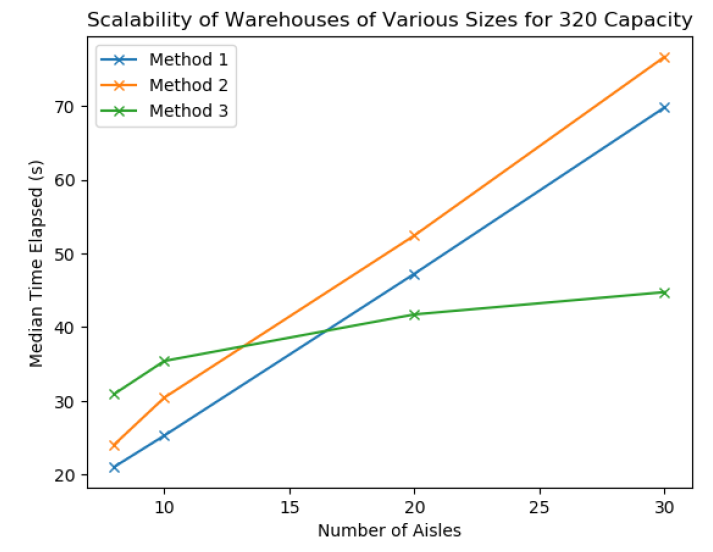
Another important yet surprising finding in our experimental results is that the median time taken for Method 3’s solving is the lowest for warehouses with 20 and 30 aisles as compared to 8 and 10 aisles. At this point in time, we are not able to explain why that is the case for Method 3, but it may be possible that the number of aisles also had a role in influencing the batching process (besides the savings router which differs across methods).

We also looked into how large an impact varying the number of blocks of each warehouse instance has on the median total distance traveled. Like with the case for median time elapsed, we analyzed each method of solving as a whole, across all the savings routers.

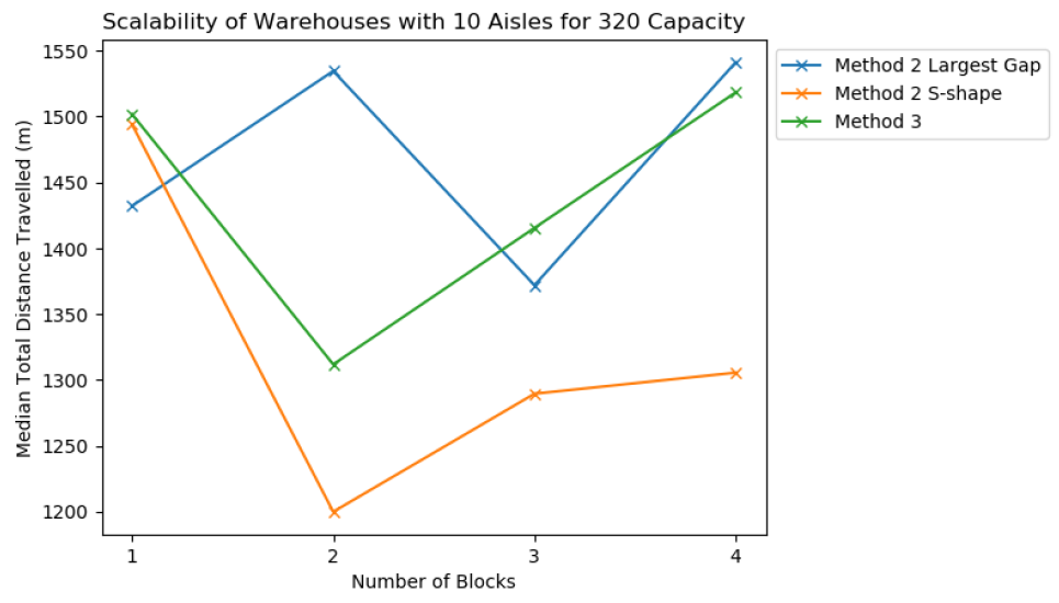
From the results collected, we observed no clear result across Methods 2 and 3 when the number of blocks for each warehouse instance was varied. Increasing the number of blocks does not lead to a consistent increase (resp. decrease) in median total distance traveled. An interesting observation we made is that there are several warehouse instances having Method 2 (with either S-shape or Largest Gap router) produce a solution with a lower median total distance traveled than Method 3. An example can be found in Figure 5.10 above, where Method 2 with S-shape router produced a lower median total distance traveled than Method 3 across all blocks for a warehouse with 10 aisles.

References

[1] Cristiano Arbex Valle, John E. Beasley, and Alexandre Salles da Cunha. Optimally solving the joint order batching and picker routing problem. European Journal of Operational Research, 262(3):817 – 834, 2017.

[2] Kees Jan Roodbergen and RenÉde Koster. Routing methods for warehouses with multiple cross aisles. International Journal of Production Research, 39(9):1865–1883, 2001.

[7] Wolsey L. A. Integer programming. 1998.

[9] David L. Applegate, Robert E. Bixby, Vasek Chvatal, and William J. Cook. The Traveling Salesman Problem: A Computational Study (Princeton Series in Applied Mathematics). Princeton University Press, Princeton, NJ, USA, 2007.